Faq/Calc/115
TDF LibreOffice Document Liberation Project Community Blogs Weblate Nextcloud Redmine Ask LibreOffice Donate
How to have more than three conditions in a conditional format
Conditional formating ( ▸ ▸ ) allows you to apply predefined styles automatically, when certain conditions are fulfilled.
For earlier versions, you can specify by default up to three conditions for checking the values in cells or formulas. The conditions are numbered 1 to 3. If condition 1 is satisfied, the defined style is used. Otherwise, condition 2 is evaluated and its style is used. If this style does not match, condition 3 is evaluated.
Here is a way to set more than 3 conditions.
Using four styles
The conditional format can set up to four different styles using this trick :
- Apply one of the four styles to the whole area : this will be the default style.
- Use the conditional formatting tool to define the conditions for applying the other three styles.
Using more than four styles
We will use the possibility of defining the format as a function of the result of a formula.
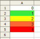
- Create as many styles as you require for the formats. In our example, we will create four cell styles, in which the only difference is the color of the background, according to the name of the style : green, yellow, orange and red. We want to conserve the Default style for the cells that do not have a whole value between 1 and 4. The result expected :
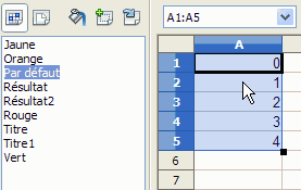
- Select the area to be formatted. After selection of a range, the first cell selected remains the current cell.
- Go to ▸ ▸
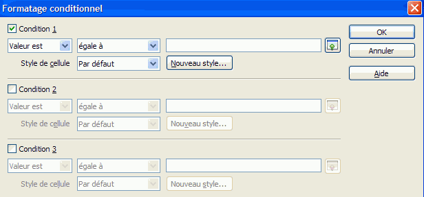
- Check Condition 1 and select Formula is.
- In the adjacent area, type the formula :
STYLE(SI(A1=1;"green";SI(A1=2;"yellow";SI(A1=3;"orange";SI(A1=4;"red";"Default")))))
Note :
- We have selected A1:A5, A1 is the current cell (see above) ; the formula refers only to A1 but the program extends the formula to the other cells selected. Relative references are used (so the second line refers to A2, etc.).
- The STYLE function is not sensitive to the case in style names. Thus, if the styles red and Red exist, the functions STYLE("Red"), STYLE("RED") or STYLE("red") all apply the same style, depending on the order in which they were created.
- You must not begin the formula with an equals (=) sign


